
This is a step-by-step guide to creating a family tree in Google Sheets.
This tree goes back five generations to great-great-grandparents. It fits on a single printed page.
You can leave out the last level for a four-generation tree.
If you’re too busy for the fifteen steps in this tutorial, jump down to the end to grab our “done for you” Google Sheets template bundle.
Table of Contents
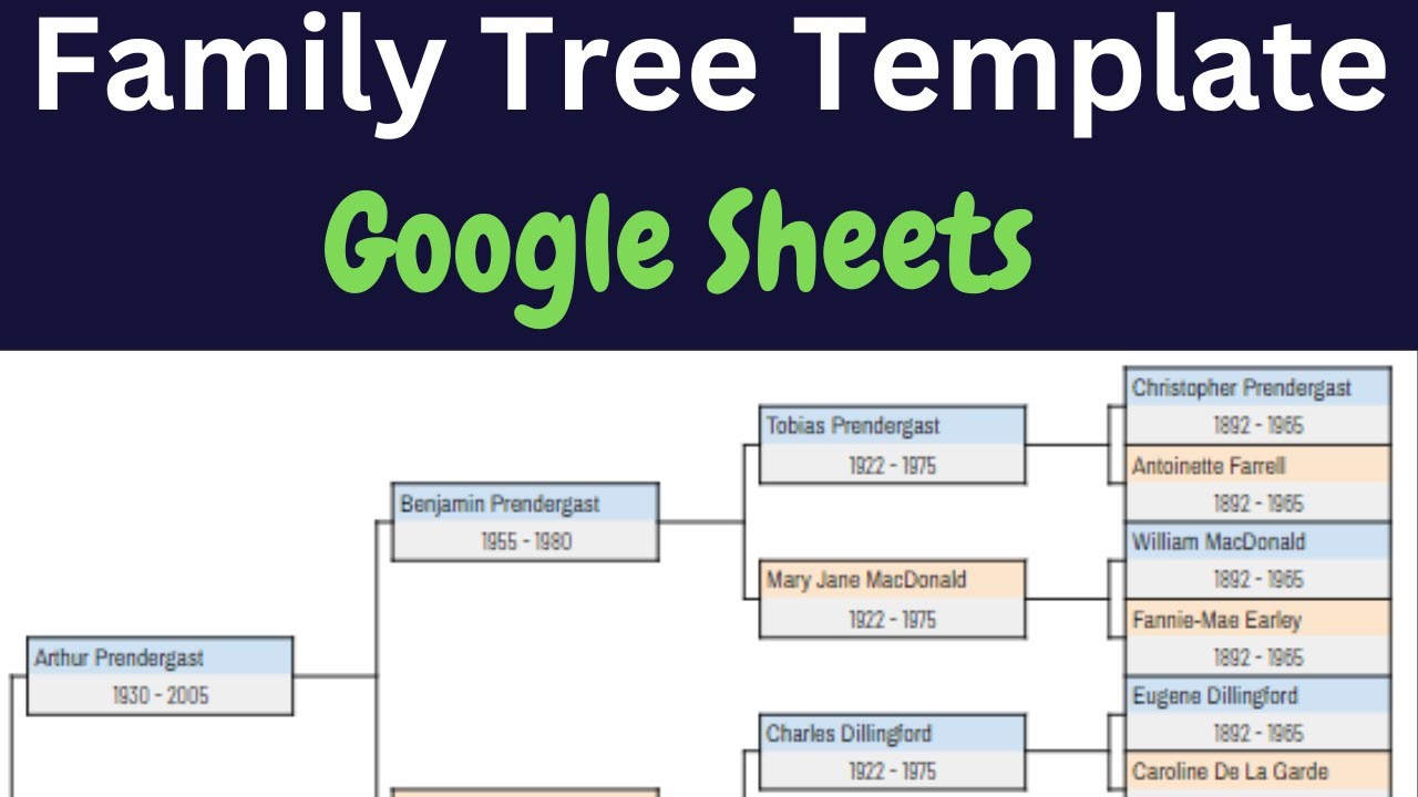
Here is what the tree looks like in Google Sheets:
I’ve left enough space in the template for a photo to the left of every person.
The individual entries look like this:

If you want one more generation that still fits on a single page, check out our guide on creating a six-generation Google Sheets family tree.
If you want one less, then here is our four generation Google Sheets template.
If you’d prefer one that’s twice the size, we have a guide to creating a ten-generation family tree in Google Sheets.
In between those two sizes, we also cover:
If you prefer a video walkthrough, click on the play button:
I’m assuming that you have a Google account. If not, sign up – it’s free.
Create a blank spreadsheet at this link.
By default, a new sheet prints as an A4 sheet in landscape mode. That’s exactly what we want.
It took a few tries to work out the best column widths to get the tree to print on a single page.
To change the width of any column, follow these steps:
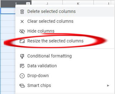
To set the width of multiple columns together, hold down the Ctrl key while clicking the column letters.
Now you know how to do it, set these widths (in pixels):
We’ll create a box to hold the name and dates for the first person.
We only need to do this once. Then we can copy the formatted cells for the other thirty people.
Place a border around cells B16 and B17 with these steps:

Arial is the default font in Google Sheets.
I find that this font is too wide to ensure that most longer names fit into the box.
My preference is to use a narrower font. These are some good choices:
Test several to see which one you find most legible at a size of 10. “Archivo Narrow” is my favorite here.
The cell beneath the name holds the dates e.g. “1923 – 1980”.
I like to have a visual difference between the name and date font.
So, I set the font for cell B17 to “Barlow Condensed”. It’s a little narrower and lighter than Archivo Narrow.
I also like the date cell to be centered. So, set the horizontal alignment to Center.
We want to ensure that a long name doesn’t spill into the next cell. The display should truncate the name to the width that we specified.
In other words, the name “Archibald Thoroughoodlivingstone” will display as “Archibald Thoroughoodliving”.
The guaranteed way is to add a space into the cell beside it.
In other words, click into cells C16 and C17 and enter a space.
The first paternal ancestor is the father.
Thankfully, we don’t have to repeat the steps above. We simply use copy-and-paste with one extra step.
When you copy the cells, don’t forget to include the ones with the space.
Unless you entered a sample name into the first name area, all you’ll see now are the bordered cells.
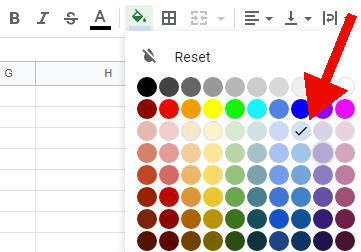
The next step is to set the background color(s) for a male ancestor. I like to use a light-blue.
To change the color of the name field:
I like to use a light gray shade for the date field below the name.

Now that we’ve got the colors set up, we can copy the newly formatted four cells to create the rest of the male ancestors.
Select and copy the four cells E8, F8, E9, and F9.
Paste into the cells below, working through them one by one:
We are now going to create the area for the mother.
In summary, we’ll copy the four cells for the father to the mother area and change the background color.
I like to set the background color for female names to “light orange 3”.
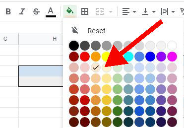
I keep the date field the same color as for the male box.
Now that we’ve got the colors set up, we can copy the newly formatted four cells to create the rest of the female ancestors.
Select and copy the four cells E24, F24, E25, and F25.
Paste into the cells below, working through them one by one:
We didn’t apply any color formatting to the home person in cells B16 and B17.
That’s because I don’t know if you’re working with a male or female person.
Follow the steps I’ve outlined to set the name and date colors appropriately.
Once that’s done, the next steps are to add the connector lines.
You can insert lines in Google Sheets and position them on the page. That’s how I prepare trees in Microsoft Excel.
But I find that lines in Google Sheets are very difficult to size precisely. The feature seems to be half-baked.
So, I use a trick to simulate lines. Instead of drawing the shape, I use cell border formatting instead.
You’ll see what I mean as you follow the next set of instructions.
Create a vertical line using borders:
Create three horizontal lines using borders:
Create the first set of connector lines:
Now we have a set of connector lines around one set of ancestors, we can copy the cells down to the other ancestors in this generation.
In other words, follow these steps:
It’s that easy! We’ll be using that copy-and-paste trick a lot to complete out this layout.
Now copy these bordered cells to the other ancestors in this generation.
Now copy these bordered cells to the other ancestors in this generation.
And that’s it! You now have the pedigree five-generation family tree structure in Excel.
You can stop and work with what you’ve got i.e. add the correct names and print out the sheet.
But if you want some photos in there, let’s keep going.
In our example tree at the top of this article, we have cropped images with faces to the left of the name and date boxes.
Because the spreadsheet images must be small, you probably have some preparation and editing to do to get similar images from your family photos.
My advice is to prepare images in either of these size units:
I’ll just come right and out say this: Google Sheets does not do a good job of letting us align images on the page. Microsoft Excel is better.
But if you really want photos on your tree, here are the steps.

The image will appear on the sheet but probably not in the correct place.
Use the arrow keys to nudge it to where it should be.
Do you find that the same size of image aligns perfectly beside one ancestor but not another? Yes, it’s annoying.
When you print your tree, be sure to turn off the grid-lines.
If you want a short-cut, we have a pre-made template in Google Sheets. Everything is laid out perfectly, you just need to fill it in!
We have two versions in the spreadsheet package:
Margaret created a family tree on a genealogy website in 2012. She purchased her first DNA kit in 2017. She created this website to share insights and how-to guides on DNA, genealogy, and family research.